7. Linearity and Detection Limits
The next few parts of this guide will provide practical information for the operator in the realization and demonstration of the key performance characteristics designed into their ICP by the manufacturer.

I have personally had the opportunity to see the advancement of ICP instrumentation over the past 30 years. Current instrumentation and software provided by manufacturers has gone well beyond anything I could have imagined 30 years ago (and it costs less). In 2004 it takes $3.21 to purchase what cost $1.00 in 1975, yet during this time period the price of ICP instrumentation has gone down while the performance characteristics have improved by orders of magnitude. A 憄ersonal experience?example is the detection limit for K by ICP-OES that has gone from 0.4 ppm to 1 ppb where the 0.4 ppm detection limit was measured on an instrument that in 1975 cost 1.5 times the 2000 price of the instrument that measured the 1 ppb detection limit (taking inflation into account, the 2000 price would be one fifth the 1975 price).

Although an ICP instrument can be wheeled into a laboratory and begin collecting data the same day, the operator is encouraged to realize and demonstrate the key performance characteristics of linearity, detectability, and spectral integrity and then go on to make decisions based upon the boundaries of these performance characteristics and the limitations of the analytical problem. Defining and being able to realize your instrument抯 performance characteristic is an investment that will save time over the years to come and allow you to make the right choices.

Defining ICP Performance Characteristics

The following steps are intended as a practical guide for the determination of an ICP抯 performance characteristics:

Read the operating manual and familiarize yourself with the software, key instrumental parameters and preferred settings before the instrument is installed.
Most instruments are supplied with optimization and wavelength or mass calibration standards that will be used during set-up by the service technician and are intended for use on a regular basis by the operator. Discuss the optimization process with the manufacturer as well as the preferred settings for the key instrumental parameters.

The remaining steps assume that the operator fully understands and is able to perform the optimization process that has been defined by the manufacturer as well as the spectral limitations of the instrument.
Select the lines to be studied for each element (憀ines?is used in this document to mean either wavelength or mass).
Line selection is based upon spectral interference issues, detection limit requirements and working range requirements. Select as many lines as possible within practicality for each element. The greater the number of lines, the greater the flexibility.
Prepare single element standards over the anticipated working range for each element. The range of standards depends upon the analytical requirements. The following ranges are suggestions only:

• Radial view ICP-OES: 0.0, 1, 10, 100, and 1000 礸/mL
• Axial view ICP-OES: 0.0, 0.1, 1, 10, and 100 礸/mL
• Quadrupole (R~ 300) mass filtered ICP-MS: 0, 1, 10, 100, and 1000 ng/mL

This step is important because these data can be used to determine instrument detection limits (IDL), linear working ranges, and spectral characteristics such as background equivalent concentrations (BEC) and spectral interferences. With most modern (if not all) instruments, the spectra obtained for each element at each concentration can be saved for review later. In addition, the software will calculate the IDL and BEC plus the linear regression of each line will establish the linear working range. All of this is typically done for the operator by the software that comes with the instrument. If at all possible, attempt to:

Use single element standards that have the trace metals impurities reported on the certificate of analysis. Most chemical standards manufacturers provide this information with their single element standards. These data are important in identifying direct spectral overlap interferences and in not identifying an impurity as an interference of this type.

Store all spectra on computer and collect the spectra for all lines of interest on each and every solution. This means that if you are interested in possibly using up to 6 lines for roughly 72 elements, then each solution spectrum totaling 72 x 6 = ~ 432 lines per solution and ~ 432 x 5 = 2160 spectra for each element need to be stored for future reference. Most ICP-MS applications would require far fewer data to be collected due to the reduced number of lines available and/or feasible.

Wash blank acid solution through the instrument for several minutes 慴etween elements?and always analyze a blank at the beginning of each element concentration series. Look for the presence of the prior element analyzed to confirm that it has been completely washed out of the introduction system.

Having the data available on a desktop computer is convenient and allows the analyst to construct potential spectra by calling up the element and the anticipated concentration for each element in the analytical sample. Having several lines available makes the job of line selection easy as well as the estimation of the line抯 sensitivity and linearity. Constructing these composite spectra from pure single element solutions eliminates confusion as to the identity of the line. The following example is intended to illustrate the process:

Examples of Spectra:

NOTE: All spectra were obtained using a concentric glass nebulizer with no problems around salting out or plugging.

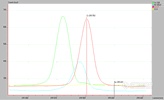
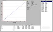
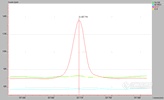
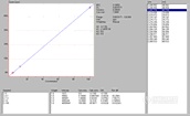
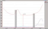
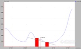
The following example is for an application where a submitter has been obtaining minor levels (0.1 to 1.0 %) of Cr in an alloy containing roughly equal amounts of Fe and Ni. The laboratory where this alloy is analyzed uses a procedure where 0.2 grams of the sample is dissolved in 5 mL of a 1:1 HNO3 / HCl mixture and diluted to 1000 mL with DI water. The analyst is informed that a limit of detection (LOD = 3SD0) of 1 ppm Cr based upon the original sample and the ability to quantify the Cr to within &plmn;10 % relative at the 10 ppm level is an absolute minimum requirement.

The submitter then asks the analyst the usual question, 揑 need the results tomorrow ?can you do it??The analyst does a quick calculation and determines that using the most sensitive Cr line and the current procedure, the lowest possible detection limit is 4 ppm and a more realistic estimation would be ~ 4 times the IDL or ~ 16 ppm. The analyst then pulls up the following spectra, instrument detection limits, and linear regression data which were obtained on their radial view instrument about four years ago when installed using pure single element solutions as described above.

0
赞贴
2
回帖
0
收藏
0
拍砖
版主
招募

为您推荐

近期热榜

热门活动

您可能想找: ICP-AES/ICP-OES 询底价

选参数看心得找厂商查方案

专属顾问快速对接

立即提交

相关阅读

tzl75

结帖率：

100%

关注：0 |粉丝：0

新手级：新兵

2005/3/24 19:19:00 沙发管理分享倒序浏览只看楼主回复私聊

The 205.552 nm Cr line was found to be the most sensitive of the 16 Cr lines originally characterized with an IDL of 4.0 ppm = [ (0.0008 礸/mL Cr IDL) x 1000 ] / 0.2 based upon original sample size and dilution as described above. However, the spectrum of a 0.1 ppm Cr standard shows significant interference from both Ni and Fe at a concentration of 100 ppm making the line useless at low ppm Cr levels (see Figures 7.1 and 7.2).

Figure 7.1:
Spectra of pure 100 ppm Fe and Ni solutions, 0.1 ppm Cr and a water blank at the 205.552 nm Cr wavelength

Figure 7.2:
IDL, BEC and regression data for the 205.552 nm Cr line

The analyst then begins the relatively simple process of identifying a Cr line with the most sensitivity that is spectrally clean. Figures 7.3 and 7.4 show the line identified using the same scan data shown for the 205 Cr line. The 267.716 nm Cr line looks clean at the current dilution factors and has an IDL of 0.0016 礸/mL Cr which increases the detection limit to somewhere between 8 to 32 ppm.

Figure 7.3:
Spectra of pure 100 ppm Fe and Ni solutions, 0.1 ppm Cr and a water blank at the 267.716 nm Cr wavelength

Figure 7.4:
IDL, BEC and regression data for the 267.716 nm Cr line

The good news is that the 267.716 line looks spectrally clean and the possibility of increasing the sample size while lowering the final volume by a factor of 100 is possible (i.e., 2 grams sample up to 100 mL using 20 mL of 1:1 HCl/ HNO3). The concentrations of the Fe and Ni in the final solution would be ~ 10,000 礸/mL each. This capability was confirmed when 40,000 礸/mL solutions of both Fe and Ni were scanned as shown in Figure 7.5. These spectral data indicate a realistic detection of << 1 ppm Cr.

Figure 7.5:
Spectra of pure 40,000 ppm Fe and Ni solutions, 0.1 ppm Cr and a water blank at the 267.716 nm Cr wavelength

Figure 7.6:
Simulated spectrum of a solution produced from 2 grams 100 mL solution of a 50/50 wt. % Ni/Fe alloy containing 1.25 ppm Cr at the 267.716 nm Cr wavelength

The spectra in Figure 5 were used to artificially produce Figure 6 which approximates signals that would be measured for a Fe/Ni alloy where 2 grams to 100 mL dilution were made on a sample containing 1.25 ppm Cr. The entire investigation was performed using spectra that had been stored on computer (i.e., the analyst can literally provide an answer as to project feasibility while speaking on the phone with the client).

The above process is not intended to take the place of method validation, but rather to arm the analyst with sufficient data to make intelligent choices during the initial stages of method development.

Confirm Basic Performance Criteria
The following excerpt was taken from part 17 of our Reliable Measurements series. This secsion discusses performance criteria confirmation during the method validation process. Please note that the validation process is more detailed and specific.

The method must 'fit the purpose' as agreed upon between the client and the analyst. In the case of trace analysis, the following criteria are typically evaluated as part of the method development process:

Specificity involves the process of line selection and confirmation that interferences (of the types discussed in part 15 and part 16) for the ICP-OES or ICP-MS measurement process are not significant. A comparison of results obtained using a straight calibration curve (without internal standardization to that of internal standardization and/or to the technique of standard additions) will give information concerning matrix effects, drift, stability, and the factors that influence the stability. The various types of spectral interferences encountered using ICP-MS and ICP-OES (see above links) should be explored.

Accuracy or Bias can be best established through the analysis of a certified reference material (CRM, or SRM if obtained from NIST). If a CRM is not available, then a comparison to data obtained by an independent validated method is the next best approach. If an alternate method is not available, then an inter-laboratory comparison, whereby the laboratories involved are accredited (ISO 17025 with the analysis on the scope of accreditation) is a third choice. The last resort is an attempt to establish accuracy through spike recovery experiments and/or the use of standard additions.

Repeatability (single laboratory precision) can be initially based upon one homogeneous sample and is measured by the laboratory developing the method. The repeatability is expressed as standard deviation.

Limit of Detection (LOD) is a criterion that can be difficult to establish. The detection limit of the method is defined as 3*SD0, where SD0 is the value of the standard deviation as the concentration of the analyte approaches 0. The value of SD0 can be obtained by extrapolation from a plot of standard deviation (y axis) versus concentration (x axis) where three concentrations are analyzed ~ 11 times each that are at the low, mid, and high regions of interest. This determination should be made using a matrix that matches the sample matrix.

Sensitivity or delta C = 2 (2)1/2 SDc, where SDc is the standard deviation at the mid point of the region of interest. This represents the minimum difference in two samples of concentration C that can be distinguished at the 95% confidence level.

Limit of Quantitation (LOQ) is defined as 10 SD0 and will have an uncertainty of ~ 30% at the 95% confidence level.

Linearity or Range is a property that is between the limit of quantitation and the point where a plot of concentration versus response goes non-linear.

赞贴

拍砖

Last edit by tzl75